# This cell is to allow automatic notebook generation for docs
# You may want to comment this out if you have paste3 installed
import sys
from pathlib import Path

sys.path.insert(0, str(Path.cwd().parent.parent.parent / "src"))

Using the PASTE2 algorithm

This noteook highlights the creation of slices (Anndata objects), usage of the pairwise_align and center_align functions of paste3, along with stacking and plotting functionalities.

This notebook primarily highlights how you would use the ``paste3`` package in ``PASTE2`` (i.e. partial alignment) mode, when adjacent slices do not fully overlap in space or have different cell type compositions.

import matplotlib.patches as mpatches
import matplotlib.pyplot as plt
import numpy as np
import scanpy as sc
import seaborn as sns

from paste3 import paste, visualization

Read in Spatial Transcriptomics slices as AnnData objects

We provide four example ST slices from DLPFC patient 3, cropped to form partially overlapping subslices (See Figure 3A of our paper). Each slice is stored in an AnnData object.

sliceA_filename = "../../../tests/data/151673.h5ad"
sliceB_filename = "../../../tests/data/151674.h5ad"
sliceC_filename = "../../../tests/data/151675.h5ad"
sliceD_filename = "../../../tests/data/151676.h5ad"
sliceA = sc.read_h5ad(sliceA_filename)
sliceB = sc.read_h5ad(sliceB_filename)
sliceC = sc.read_h5ad(sliceC_filename)
sliceD = sc.read_h5ad(sliceD_filename)

Each AnnData object consists of a gene expression matrx and spatial coordinate matrix. The gene expression matrix is stored in the .X field. The spatial coordiante matrix is stored in the .obsm['spatial'] field.

sliceA.X

<Compressed Sparse Row sparse matrix of dtype 'float32'
        with 5798687 stored elements and shape (2929, 11381)>

sliceA.obsm["spatial"]

array([[ 5769,  2807],
       [ 4068,  9505],
       [ 3393,  7583],
       ...,
       [ 4631,  7831],
       [ 5571, 11193],
       [ 6317,  3291]])

The rows of the AnnData objects are spots. The columns are genes.

sliceA.obs

	in_tissue	array_row	array_col	imagerow	imagecol	sum_umi	sum_gene	subject	position	replicate	...	layer_guess_reordered_short	n_genes_by_counts	log1p_n_genes_by_counts	total_counts	log1p_total_counts	pct_counts_in_top_50_genes	pct_counts_in_top_100_genes	pct_counts_in_top_200_genes	pct_counts_in_top_500_genes	n_counts
AAACAATCTACTAGCA-1.3	1	3	43	126.327637	259.630972	1667	1150	Br8100	0	1	...	L1	1150	7.048386	1667.0	7.419381	22.975405	30.173965	42.171566	61.007798	1628.0
AAACACCAATAACTGC-1.8	1	59	19	427.767792	183.078314	3769	1960	Br8100	0	1	...	WM	1960	7.581210	3769.0	8.234830	25.975060	33.138764	42.531175	59.697533	3704.0
AAACAGCTTTCAGAAG-1.7	1	43	9	341.269139	152.700275	4278	2264	Br8100	0	1	...	L5	2264	7.725330	4278.0	8.361475	23.796166	30.201029	38.826554	54.698457	4217.0
AAACAGGGTCTATATT-1.8	1	47	13	362.916304	164.941500	4004	2178	Br8100	0	1	...	L6	2178	7.686621	4004.0	8.295299	24.600400	30.669331	39.185814	55.344655	3922.0
AAACAGTGTTCCTGGG-1.5	1	73	43	503.780395	256.930702	2376	1432	Br8100	0	1	...	WM	1432	7.267525	2376.0	7.773594	26.136364	33.501684	43.308081	60.774411	2339.0
...	...	...	...	...	...	...	...	...	...	...	...	...	...	...	...	...	...	...	...	...	...
TTGTTTCACATCCAGG-1.8	1	58	42	422.862301	254.410450	4324	2170	Br8100	0	1	...	WM	2170	7.682943	4324.0	8.372168	22.941721	30.388529	40.703053	57.770583	4266.0
TTGTTTCATTAGTCTA-1.8	1	60	30	433.393354	217.146722	2761	1560	Br8100	0	1	...	WM	1560	7.353082	2761.0	7.923710	26.439696	34.190511	43.824701	61.608113	2715.0
TTGTTTCCATACAACT-1.8	1	45	27	352.430255	208.415849	2322	1343	Br8100	0	1	...	L6	1343	7.203406	2322.0	7.750615	31.093885	37.941430	47.243755	63.695090	2300.0
TTGTTTGTATTACACG-1.4	1	73	41	503.735391	250.720081	2331	1420	Br8100	0	1	...	WM	1420	7.259116	2331.0	7.754481	25.139425	32.947233	42.728443	60.531961	2286.0
TTGTTTGTGTAAATTC-1.8	1	7	51	148.109816	284.293439	6281	2927	Br8100	0	1	...	L2	2927	7.982075	6281.0	8.745443	24.231810	30.154434	38.242318	53.017036	6184.0

2929 rows × 24 columns

sliceA.var

	gene_ids	feature_types	genome	n_cells_by_counts	mean_counts	log1p_mean_counts	pct_dropout_by_counts	total_counts	log1p_total_counts	n_counts
NOC2L	ENSG00000188976	Gene Expression	GRCh38	690	0.223963	0.202094	81.038747	815.0	6.704414	815.0
KLHL17	ENSG00000187961	Gene Expression	GRCh38	163	0.045342	0.044344	95.520747	165.0	5.111988	165.0
HES4	ENSG00000188290	Gene Expression	GRCh38	875	0.303105	0.264750	75.954933	1103.0	7.006695	1103.0
ISG15	ENSG00000187608	Gene Expression	GRCh38	968	0.318494	0.276490	73.399286	1159.0	7.056175	1159.0
AGRN	ENSG00000188157	Gene Expression	GRCh38	1038	0.351470	0.301193	71.475680	1279.0	7.154615	1279.0
...	...	...	...	...	...	...	...	...	...	...
MT-ND4	ENSG00000198886	Gene Expression	GRCh38	3639	85.596596	4.461260	0.000000	311486.0	12.649113	311486.0
MT-ND5	ENSG00000198786	Gene Expression	GRCh38	3593	9.799670	2.379516	1.264084	35661.0	10.481841	35661.0
MT-ND6	ENSG00000198695	Gene Expression	GRCh38	1966	0.860126	0.620644	45.974169	3130.0	8.049108	3130.0
MT-CYB	ENSG00000198727	Gene Expression	GRCh38	3639	49.170376	3.915425	0.000000	178931.0	12.094761	178931.0
AC007325.4	ENSG00000278817	Gene Expression	GRCh38	577	0.183567	0.168533	84.143996	668.0	6.505784	668.0

11381 rows × 10 columns

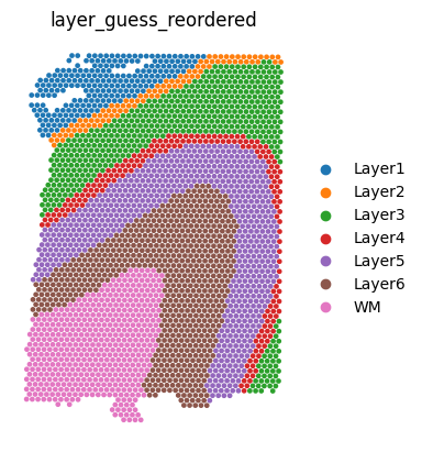
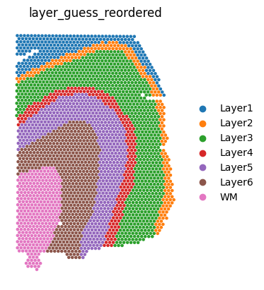
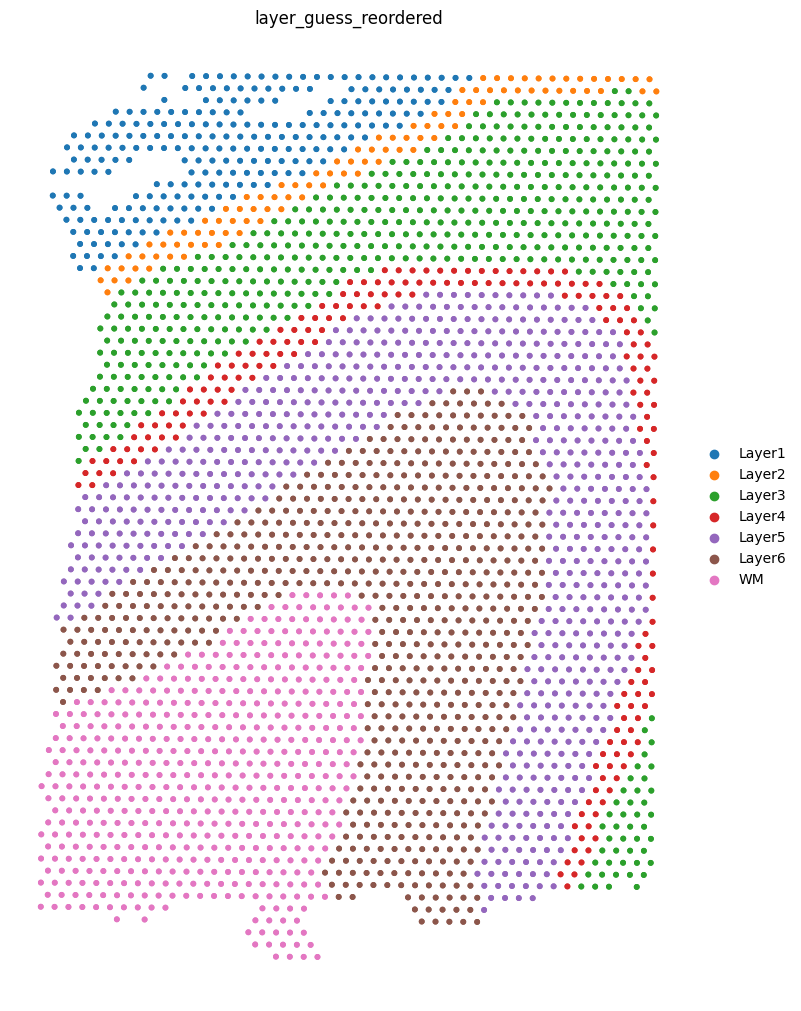
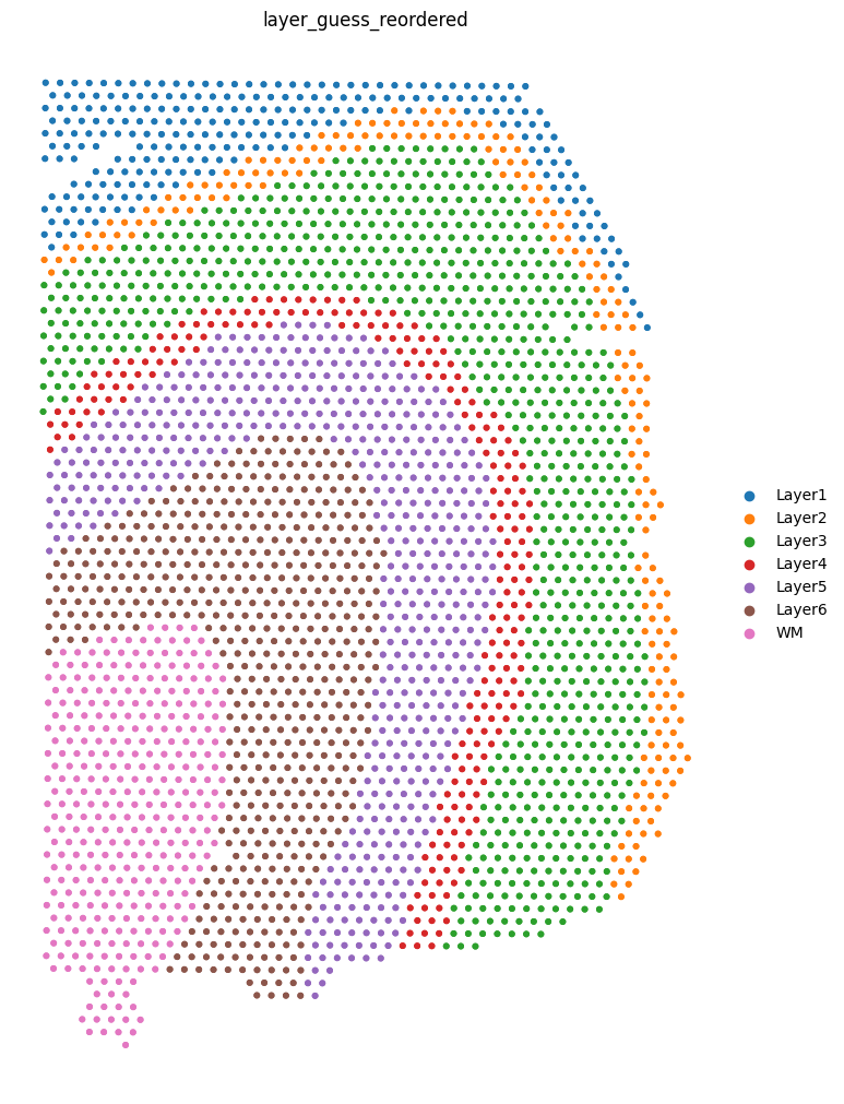
We can visualize the slices using scanpy. In this case, the .obs["layer_guess_reordered"] field stores the layer annotation of each slice, so we use this field to color each spot.

sc.pl.spatial(sliceA, color="layer_guess_reordered", spot_size=125, frameon=False)
sc.pl.spatial(sliceB, color="layer_guess_reordered", spot_size=125, frameon=False)
sc.pl.spatial(sliceC, color="layer_guess_reordered", spot_size=125, frameon=False)
sc.pl.spatial(sliceD, color="layer_guess_reordered", spot_size=125, frameon=False)

Compute partial pairwise alignment using PASTE2

Give a pair of partially overlapping slices, we can use partial_pairwise_align() to find an alignment matrix. To call the function, you need to input the AnnData objects of the two slices, as well as a parameter s, which indicates the overlap percentage of the two slices. In this tutorial, each pair of cropped subslices overlap at 70% of the areas, so we set overlap_fraction=0.7. For your own datasets you should visualize the slices and manually determine the approximate overlap percentage (this parameter does not have to be very accurate).

Now we compute an alignment matrix between each pair of slices in our example dataset.

In the calls to ``pairwise_align`` below, we’re using maxIter=20 here to specify a maximum of 20 iterations for pairwise_align. This is only to allow this demo to run in a resonable amount of time. In a real alignment scenario, you should not include this argument.

pi_AB, _ = paste.pairwise_align(sliceA, sliceB, overlap_fraction=0.7, maxIter=20)

(INFO) (paste.py) (10-Jan-25 17:08:25) GPU is not available, resorting to torch CPU.

pi_BC, _ = paste.pairwise_align(sliceB, sliceC, overlap_fraction=0.7, maxIter=20)

(INFO) (paste.py) (10-Jan-25 17:10:17) GPU is not available, resorting to torch CPU.

pi_CD, _ = paste.pairwise_align(sliceC, sliceD, overlap_fraction=0.7, maxIter=20)

(INFO) (paste.py) (10-Jan-25 17:12:04) GPU is not available, resorting to torch CPU.

Let’s check the shape of each alignment matrix. For aligning a slice with n1 spots and a slice with n2 spots, the alignment matrix should be of shape (n1 * n2)

print(pi_AB.shape)
print(pi_BC.shape)
print(pi_CD.shape)

torch.Size([2929, 2877])
torch.Size([2877, 2873])
torch.Size([2873, 2701])

There are other optional parameters to PASTE2.partial_pairwise_align() as well. You can checkout the original function signature in the souce code with documentation.

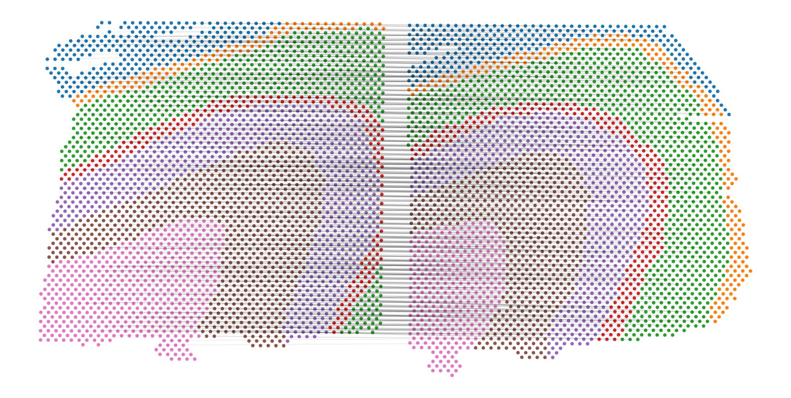
Let’s visualize the alignment between sliceA and sliceB:

def largest_indices(ary, n):
    """Returns the n largest indices from a numpy array."""
    flat = ary.flatten()
    indices = np.argpartition(flat, -n)[-n:]
    indices = indices[np.argsort(-flat[indices])]
    return np.unravel_index(indices, ary.shape)


def plot2D_samples_mat(xs, xt, G, alpha=0.2, top=1000, weight_alpha=False, **kwargs):
    if ("color" not in kwargs) and ("c" not in kwargs):
        kwargs["color"] = "k"
    mx = G.max().item()
    #     idx = np.where(G/mx>=thr)
    idx = largest_indices(G.cpu().numpy(), top)
    for i in range(len(idx[0])):
        plt.plot(
            [xs[idx[0][i], 0], xt[idx[1][i], 0]],
            [xs[idx[0][i], 1], xt[idx[1][i], 1]],
            alpha=alpha * (1 - weight_alpha)
            + (weight_alpha * G[idx[0][i], idx[1][i]].item() / mx),
            c="k",
        )


def plot_slice_pairwise_alignment(
    slice1, slice2, pi, alpha=0.05, top=1000, weight_alpha=False
):
    coordinates1, coordinates2 = slice1.obsm["spatial"], slice2.obsm["spatial"]
    offset = (coordinates1[:, 0].max() - coordinates2[:, 0].min()) * 1.1
    temp = np.zeros(coordinates2.shape)
    temp[:, 0] = offset
    plt.figure(figsize=(20, 10))
    plot2D_samples_mat(
        coordinates1,
        coordinates2 + temp,
        pi,
        c="k",
        alpha=alpha,
        top=top,
        weight_alpha=weight_alpha,
    )
    plt.scatter(
        coordinates1[:, 0],
        coordinates1[:, 1],
        linewidth=0,
        s=100,
        marker=".",
        color=list(
            slice1.obs["layer_guess_reordered"].map(
                dict(
                    zip(
                        slice1.obs["layer_guess_reordered"].cat.categories,
                        slice1.uns["layer_guess_reordered_colors"],
                        strict=False,
                    )
                )
            )
        ),
    )
    plt.scatter(
        coordinates2[:, 0] + offset,
        coordinates2[:, 1],
        linewidth=0,
        s=100,
        marker=".",
        color=list(
            slice2.obs["layer_guess_reordered"].map(
                dict(
                    zip(
                        slice2.obs["layer_guess_reordered"].cat.categories,
                        slice2.uns["layer_guess_reordered_colors"],
                        strict=False,
                    )
                )
            )
        ),
    )
    plt.gca().invert_yaxis()
    plt.axis("off")
    plt.show()


plot_slice_pairwise_alignment(sliceA, sliceB, pi_AB)

Project all slices onto the same coordiante system according to the alignment

Once the alignment matrix between each pair of adjacent slices in a sequence of consecutive slices are computed, we can use this information to project all slices onto the same 2D coordinate system. 3D reconstruction can be done by assiging a z-coordiante to each slice after the projection.

Specifically, we use visualization.partial_stack_slices_pairwise( ):

pis = [pi_AB, pi_BC, pi_CD]
slices = [sliceA, sliceB, sliceC, sliceD]

new_slices, _, _ = visualization.stack_slices_pairwise(slices, pis, is_partial=True)

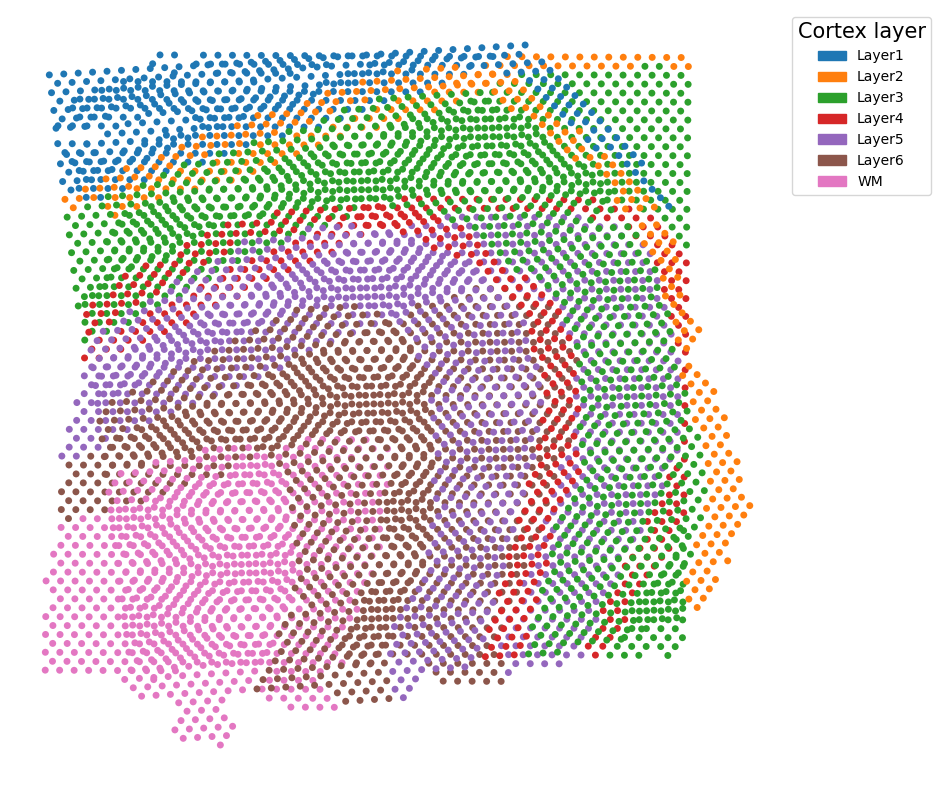
Now let’s plot the coordinates of all slices after the projection:

layer_to_color_map = {f"Layer{i + 1}": sns.color_palette()[i] for i in range(6)}
layer_to_color_map["WM"] = sns.color_palette()[6]


def plot_slices_overlap(slices, layer_to_color_map=layer_to_color_map):
    plt.figure(figsize=(10, 10))
    for i in range(len(slices)):
        adata = slices[i]
        colors = list(
            adata.obs["layer_guess_reordered"].astype("str").map(layer_to_color_map)
        )
        plt.scatter(
            adata.obsm["spatial"][:, 0],
            adata.obsm["spatial"][:, 1],
            linewidth=0,
            s=100,
            marker=".",
            color=colors,
        )
    plt.legend(
        handles=[
            mpatches.Patch(
                color=layer_to_color_map[
                    adata.obs["layer_guess_reordered"].cat.categories[i]
                ],
                label=adata.obs["layer_guess_reordered"].cat.categories[i],
            )
            for i in range(len(adata.obs["layer_guess_reordered"].cat.categories))
        ],
        fontsize=10,
        title="Cortex layer",
        title_fontsize=15,
        bbox_to_anchor=(1, 1),
    )
    plt.gca().invert_yaxis()
    plt.axis("off")
    plt.show()


plot_slices_overlap(new_slices)

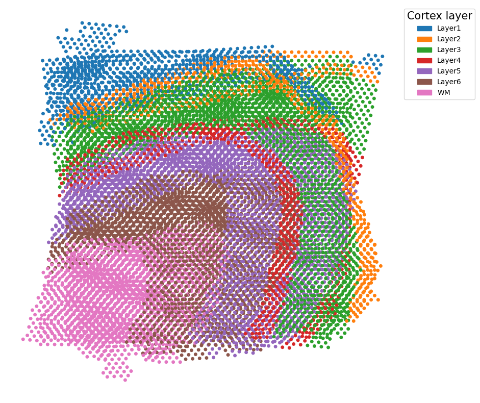
Or just the first two, which reproduces Figure 3C of the paper:

plot_slices_overlap(new_slices[:2])